A Basic Guide to Testing the Assumptions of Linear Regression in R

The very first step after building a linear regression model is to check whether your model meets the assumptions of linear regression. These assumptions are a vital part of assessing whether the model is correctly specified. In this blog I will go over what the assumptions of linear regression are and how to test if they are met using R.

Let’s get started!

What are the Assumptions of Linear Regression?

There are primarily five assumptions of linear regression. They are:

1. There is a linear relationship between the predictors (x) and the outcome (y)
2. Predictors (x) are independent and observed with negligible error
3. Residual Errors have a mean value of zero
4. Residual Errors have constant variance
5. Residual Errors are independent from each other and predictors (x)

How to Test the Assumptions of Linear Regression?

In this section I will show you how to test each of the assumptions in R. I am using R studio version 1.4.1103. Also, prior to testing the assumptions, you must have a model built out.

Assumption One: Linearity of the Data

We can check the linearity of the data by looking at the Residual vs Fitted plot. Ideally, this plot would not have a pattern where the red line (lowes smoother) is approximately horizontal at zero.

Here is the code: plot(model name, 1)

This is what we want to see:

This is what we don’t want to see:

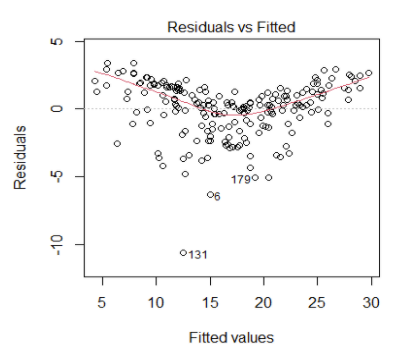
In the above plot, we can see that there is a clear pattern in the residual plot. This would indicate that we failed to meet the assumption that there is a linear relationship between the predictors and the outcome variable.

Assumption Two: Predictors (x) are Independent & Observed with Negligible Error

The easiest way to check the assumption of independence is using the Durbin-Watson test. We can conduct this test using R’s built-in function called durbinWatsonTest on our model. Running this test will give you an output with a p-value, which will help you determine whether the assumption is met or not. 

Here is the code: durbinWatsonTest(model name)

The null hypothesis states that the errors are not auto-correlated with themselves (they are independent). Thus, if we achieve a p-value > 0.05, we would fail to reject the null hypothesis. This would give us enough evidence to state that our independence assumption is met!

Assumption Three: Residual Errors have a Mean Value of Zero

We can easily check this assumption by looking at the same residual vs fitted plot. We would ideally want to see the red line flat on 0, which would indicate that the residual errors have a mean value of zero.

In the above plot, we can see that the red line is above 0 for low fitted values and high fitted values. This indicates that the residual errors don’t always have a mean value of 0.

Assumption Four: Residual Errors have Constant Variance

We can check this assumption using the Scale-Location plot. In this plot we can see the fitted values vs the square root of the standardized residuals. Ideally, we would want to see the residual points equally spread around the red line, which would indicate constant variance.

Here is the code: plot(model name, 3)

This is what we want to see:

This is what we don't want to see:

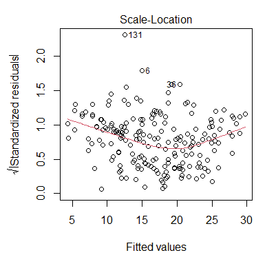
In the above plot, we can see that the residual points are not all equally spread out. Thus, this assumption is not met. One common solution to this problem is to calculate the log or square root transformation of the outcome variable. 

We can also use the Non-Constant Error Variance (NVC) Test using R’s built in function called nvcTest to check this assumption. Make sure you install the package car prior to running the nvc test.

Here is the code: nvcTest(model name)

This will output a p-value which will help you determine whether your model follows the assumption or not. The null hypothesis states that there is constant variance. Thus, if you get a p-value> 0.05, you would fail to reject the null. This means you have enough evidence to state that your assumption is met!

Assumption Five: Residual Errors are Independent from Each Other & Predictors (x)

This assumption requires knowledge of study design or data collection in order to establish the validity of this assumption, so we will not be covering this in this blog.

And there you have it! 

While this is only a short list, these are my preferred ways to check linear assumptions! I hope this blog answered some of your questions and helped you in your modeling journey!

Start your data journey with our Analytics Accelerator program